数学建模

数学知识点

高等数学-多元微积分-空间曲线

Wang Haihua

🚅 🚋😜 🚑 🚔

Visualizing a space curve¶

Vector Functions on Intervals

When a particle moves through space during a time interval $I$, we think of the particle's coordinates as functions defined on $I$:

\begin{equation} x = f(t), \ y = g(t),\ z = h(t) \ \ \ \mbox{for}\ \ t\in I = [a, b]. \end{equation}

The points $(x, y, z) = (f(t), g(t), h(t))$ make up the curve in space that we call a particle's path.

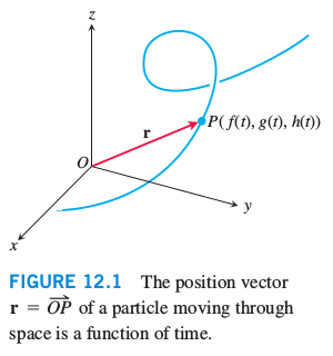
A curve in space can also be represented in vector form: \begin{equation} \vec{r}(t) = f(t)\vec{i}+g(t)\vec{j}+h(t)\vec{k} = <f(t), g(t), h(t)> \end{equation} where $\vec{i}, \vec{j}$, and $\vec{k}$ are standard unit vectors.

Equation (2) defines $\vec{r}$ as a vector function of the real variable $t$ on the interval $I$. More generally, a vector-valued function or vector function on a domain set $D$ is a rule that assigns a vector in space to each element in $D$. For now, the domains will be intervals of real numbers resulting in a space curve. Domains can be regions in the plane. Vector functions will then represent surfaces in space. Vector functions on a domain in the plane or space also give rise to vector fields, which are important to the study of the flow of a fluid, gravitational fields, and electromagnetic phenomena.

We want to visualize vectors functions on intervals using a python package Sympy.

In [12]:

# Import necessary packages
%matplotlib inline
from sympy import symbols, cos, sin
from sympy.plotting import plot3d_parametric_line as ppl3
from sympy.plotting import plot_parametric as ppl
import numpy as np

t = symbols('t')

Example 1 Visualize $\vec{r}(t) = <t^2-3t, t+2>$ for $t\in [-2\pi, 3\pi]$.

In [13]:

ppl(t**2-3*t, t+2, (t, -2*np.pi, 3*np.pi))

Out[13]:

<sympy.plotting.plot.Plot at 0x7f65b3ccf898>

Example 2 Visualize $\vec{r}(t) = \cos t\,\vec{i} + \sin t\,\vec{j} + t\,\vec{k}$ for $t\in [0, 6\pi]$.

In [14]:

ppl3(cos(t), sin(t), t, (t, 0, 6*np.pi))

Out[14]:

<sympy.plotting.plot.Plot at 0x7f65b3b6df98>

Exercises

Visualize vector functions.

$\vec{r}(t) = (\sin 3t)(\cos t)\vec{i} + (\sin 3t)(\sin t)\vec{j} +t\vec{k}$
$\vec{r}(t) = (\cos t)\vec{i} + (\sin t)\vec{j} + (\sin 2t)\vec{k}$
$\vec{r}(t) = (4+\sin 20t)(\cos t)\vec{i} + (4+\sin 20t)(sin t) + (\cos 20t)\vec{k}$